The Geometry of Invisible Waves: Anatomy of a Radar and FMCW Mathematics
The art of encoding time into frequency at the speed of light: FMCW radar hardware architecture, chirp mathematics, 2D-FFT signal processing algorithms, and millimeter-wave PCB design challenges.
1. Introduction: Racing Time at the Speed of Light
The instant you release an electromagnetic wave into free space, you enter a race with the universal speed limit: the speed of light ($c \approx 3 \times 10^8\text{ m/s}$). This velocity is difficult to grasp on macroscopic human scales: in one second, light circles the Earth seven and a half times; in a single nanosecond ($10^{-9}\text{ s}$), it travels merely 30 centimeters.
Now imagine placing a radar sensor on your desk and measuring the range to an object $1.5\text{ meters}$ away. The round-trip distance traveled by the electromagnetic pulse is $3\text{ meters}$, and the entire round-trip flight lasts only 10 nanoseconds. If the target moves by just $15\text{ centimeters}$, the resulting differential time-of-flight shift is a microscopic 1 nanosecond.
Attempting to resolve this problem using a classical Pulsed Radar (Time-of-Flight) architecture runs directly into three formidable hardware barriers:
- Blind Zones and High Peak Power: To detect proximate targets, the transmit pulse width ($\tau_p$) must be compressed down to picoseconds or a few nanoseconds. As pulse duration shrinks, the instantaneous Peak Power must be boosted into hundreds of watts or kilowatts to return measurable energy. Furthermore, the sensitive Low-Noise Amplifier (LNA) on the receive (RX) path must be blanked while the transmitter (TX) fires to prevent destruction, creating a permanent blind zone right in front of the antenna.
- Ultra-Fast ADC Requirements: Digitizing a nanosecond pulse directly in the time domain demands analog-to-digital converters operating at tens of Giga-Samples Per Second (GSPS), incurring extreme power dissipation, thermal penalties, and prohibitive bill-of-materials costs.
- Form-Factor and Integration Limits: High peak RF power levels cannot be accommodated within compact monolithic microwave integrated circuits (MMICs) manufactured in silicon CMOS or SiGe BiCMOS for automotive, robotic, and industrial sensors.
This is why modern autonomous vehicles, industrial robots, and precision distance sensors eschew pulsed systems in favor of FMCW (Frequency-Modulated Continuous Wave) radar.
💡 The FMCW Paradigm: An FMCW radar does not attempt to measure time-of-flight with a nanosecond stopwatch. Instead, it encodes time into frequency. By ramping the transmitted carrier frequency linearly over time, unmeasurable nanosecond delays ($\tau$) are mixed down into easily sampled kilohertz ($\text{kHz}$) or low megahertz ($\text{MHz}$) Beat Frequencies ($f_b$).
2. Hardware Anatomy of an FMCW Radar
The RF front-end and baseband signal chain of an FMCW radar represent an exquisite synthesis of microwave engineering and digital signal processing (DSP):
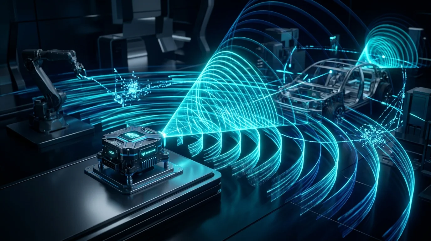 Figure: Millimeter-wave FMCW radar antenna array emitting linear frequency-modulated chirp waveforms across 3D space.
1
2
3
4
5
6
7
8
9
10
11
12
13
14
15
16
17
18
19
20
21
22
23
24
                  +-----------------------+
                  |    Chirp Synthesizer  |
                  |       (PLL + VCO)     |
                  +-----------+-----------+
                              |
                     [LO Signal: f_TX(t)]
                              |
            +-----------------+-----------------+
            |                                   |
            v                                   v
  +-------------------+               +-------------------+
  |  Power Amplifier  |               |     RF Mixer      |
  |       (PA)        |               |   (Downconverter) |
  +---------+---------+               +---------^---------+
            |                                   |
       [TX Antenna]                        [RX Signal]
            |                                   |
            v                           +-------+-------+
       )))  Wave   (((                  |   Low-Noise   |
                                        |   Amplifier   |
          [ Target ]                    |     (LNA)     |
                                        +-------^-------+
                                                |
                                           [RX Antenna]
Subsystems and Functional Roles:
- Frequency Synthesizer (Chirp Generator - PLL & VCO): The heart of the system. A Voltage-Controlled Oscillator (VCO) combined with a Fractional-N Phase-Locked Loop (PLL) generates a carrier whose frequency sweeps with high linearity ($R^2 > 0.999$). Any non-linearity in the chirp ramp causes spectral smearing and phantom target artifacts.
- Power Amplifier (PA) & TX Antenna Array: Amplifies the synthesized millimeter-wave signal (e.g., $77\text{ GHz}$) to moderate levels (typically $+10\text{ dBm}$ to $+15\text{ dBm}$, or $10-30\text{ mW}$) and radiates it via a directional microstrip patch array. Unlike pulsed radar, peak power matches average power.
- Low-Noise Amplifier (LNA): Due to path loss governed by the $1/R^4$ radar range equation, reflected echoes return attenuated down to picowatts or femtowatts. The LNA amplifies this faint signal while contributing minimal Noise Figure (NF).
- RF Mixer (Downconversion): Where the mathematical magic of FMCW occurs. The instantaneous transmit carrier (LO) is analog-multiplied with the delayed echo from the target (RX). The product of two sinusoids yields sum ($f_{TX} + f_{RX} \approx 154\text{ GHz}$) and difference ($f_{TX} - f_{RX} \sim \text{kHz}-\text{MHz}$) frequencies.
- Baseband Conditioning and ADC: A low-pass filter (LPF) discards the $154\text{ GHz}$ sum product. A tunable high-pass filter (HPF) suppresses TX-to-RX antenna leakage and strong proximate ground reflections. The resulting clean beat signal ($f_b$) is digitized by a standard ADC operating at a modest few Mega-Samples Per Second (MSPS).
3. Chirp Mathematics and Range Estimation
The fundamental waveform transmitted by an FMCW radar is a linear frequency ramp known as a Chirp. The instantaneous frequency of a Linear Frequency Modulated (LFM) chirp is expressed as:
\[f_{TX}(t) = f_c + S \cdot t \quad (0 \le t \le T_c)\]Where:
- $f_c$: Carrier start frequency (e.g., $77\text{ GHz}$),
- $T_c$: Chirp duration (e.g., $40\text{ \mu s}$),
- $B$: Sweep bandwidth (e.g., $4\text{ GHz}$, sweeping from $77\text{ GHz}$ to $81\text{ GHz}$),
- $S$: Chirp slope / ramp rate ($S = \frac{B}{T_c} = \frac{4\text{ GHz}}{40\text{ \mu s}} = 100\text{ MHz/\mu s} = 10^{14}\text{ Hz/s}$).
1
2
3
4
5
6
7
8
9
10
11
Frequency
  ^
  |        TX Signal (Transmitted)
f_c + B +      /             /
        |     /             /
        |    /             /    RX Signal (Delayed Echo)
        |   /  |<- tau ->| /
        |  /   |         |/
        | /    |         /
    f_c +/-----+--------/------------> Time
        |<-- T_c ------>|
For a stationary target located at distance $R$, the round-trip delay ($\tau$) is:
\[\tau = \frac{2R}{c}\]By the time the echo returns to the receiver, the transmitter has already swept to a higher frequency. The instantaneous frequency difference at the mixer output is the Beat Frequency ($f_b$):
\[f_b = S \cdot \tau = S \cdot \frac{2R}{c} = \frac{2 B R}{c T_c}\]This establishes the direct proportionality between range and frequency:
\[R = \frac{c T_c}{2 B} f_b = \frac{c}{2 S} f_b\]Concrete Numerical Example:
- $B = 4\text{ GHz}$, $T_c = 40\text{ \mu s}$, $S = 100\text{ MHz/\mu s}$.
- Target range $R = 15\text{ meters}$.
- Flight delay: $\tau = \frac{2 \times 15}{3 \times 10^8} = 100\text{ nanoseconds}$.
- Beat frequency: $f_b = 10^{14}\text{ Hz/s} \times 100 \times 10^{-9}\text{ s} = 10\text{ MHz}$.
A $100\text{-nanosecond}$ interval is difficult to measure directly in time; a $10\text{ MHz}$ sine wave is effortlessly digitized by an off-the-shelf $25\text{ MSPS}$ ADC.
Range Resolution ($\Delta R$):
For two adjacent targets to be resolved as distinct spectral peaks rather than a merged blur, their beat frequencies must differ by at least one FFT bin resolution ($\Delta f = 1/T_c$):
\[f_{b2} - f_{b1} \ge \frac{1}{T_c} \implies \frac{2 B \Delta R}{c T_c} \ge \frac{1}{T_c}\]Canceling $T_c$ yields the foundational radar resolution theorem:
\[\Delta R = \frac{c}{2B}\]⚠️ Key Takeaway: Range resolution is entirely independent of chirp duration and carrier frequency; it is determined solely by the RF sweep bandwidth ($B$).
- $24\text{ GHz}$ ISM band ($200\text{ MHz}$ bandwidth): $\Delta R = \frac{3 \times 10^8}{2 \times 200 \times 10^6} = 75\text{ cm}$.
- $77-81\text{ GHz}$ automotive band ($4\text{ GHz}$ bandwidth): $\Delta R = \frac{3 \times 10^8}{2 \times 4 \times 10^9} = \mathbf{3.75\text{ cm}}$. This dramatic leap in spatial resolution explains why the automotive industry abandoned 24 GHz in favor of 77 GHz radar.
4. Phase Analysis, Doppler Shift, and Velocity Estimation
If a target is moving with relative radial velocity $v$, the reflected carrier frequency shifts via the Doppler Effect:
\[f_d = \frac{2v}{\lambda} = \frac{2v f_c}{c}\]At $77\text{ GHz}$ ($\lambda \approx 3.9\text{ mm}$), an oncoming vehicle traveling at $100\text{ km/h}$ ($27.8\text{ m/s}$) generates a Doppler shift of:
\[f_d = \frac{2 \times 27.8}{0.0039} \approx 14.25\text{ kHz}\]A $14.25\text{ kHz}$ shift superimposed on a $10\text{ MHz}$ beat frequency represents a fractional variance of $\sim 0.14\%$, which cannot be extracted reliably within a single chirp.
How do modern FMCW systems measure velocity with sub-kilometer-per-hour precision? The answer lies in the Phase ($\phi$) of the beat signal.
Phase Sensitivity
The IF signal out of the mixer is modeled as:
\[s_{IF}(t) = A \cos\left( 2\pi f_b t + \phi_0 \right)\]The initial phase term ($\phi_0$) preserves the exact carrier phase over the round-trip distance:
\[\phi_0 = 2\pi f_c \tau = 2\pi f_c \left(\frac{2R}{c}\right) = \frac{4\pi R}{\lambda}\]Because $\lambda \approx 3.9\text{ mm}$, if the target displaces by merely $1\text{ millimeter}$, the phase rotates by:
\[\Delta \phi = \frac{4\pi \times 1\text{ mm}}{3.9\text{ mm}} \approx 3.22\text{ radians} \approx 185^\circ\]Sub-millimeter physical motions induce massive rotations in the IF signal’s phase.
Chirp Frame Processing
To measure velocity, the radar emits a burst of $N$ consecutive chirps separated by interval $T_c$:
1
2
3
4
5
Chirp 1         Chirp 2         Chirp 3                 Chirp N
  /               /               /                       /
 /               /               /                       /
/               /               /                       /
|<-   T_c   ->| |<-   T_c   ->| |<-   T_c   ->| ...
Between consecutive chirps, the target moves $\Delta R = v \cdot T_c$. This displacement induces a phase differential between the range peaks of successive chirps:
\[\Delta \phi = \frac{4\pi \Delta R}{\lambda} = \frac{4\pi v T_c}{\lambda} \implies v = \frac{\lambda \cdot \Delta \phi}{4\pi T_c}\]To prevent phase wrap ambiguity ($-\pi < \Delta \phi < +\pi$), the Maximum Unambiguous Velocity is:
\[v_{max} = \frac{\lambda}{4 T_c}\]The velocity resolution ($\Delta v$) across a frame of $N$ chirps is:
\[\Delta v = \frac{\lambda}{2 N T_c}\]5. Two-Dimensional FFT (2D-FFT): The Range-Doppler Heatmap
The sampled ADC data is arranged in memory as a 2D matrix (Radar Data Cube):
1
2
3
4
5
6
7
8
9
10
               Slow Time — Chirp Index (0, 1, ..., N-1)
              +--------------------------------------------------------+
              | Chirp 0 | Chirp 1 | Chirp 2 | ... | Chirp N-1          |
     +--------+---------+---------+---------+-----+--------------------+
Fast | Sample 0|        |         |         |     |                    |
Time | Sample 1|        |         |         |     |                    |
     | Sample 2|        |         |         |     |                    |
     | ...     |        |         |         |     |                    |
     | Sample M|        |         |         |     |                    |
     +--------+---------+---------+---------+-----+--------------------+
The signal processing pipeline executes across two orthogonal dimensions:
Step 1: Fast-Time FFT (Range FFT)
A 1D-FFT is performed across every column ($M$ ADC samples within a chirp). Each spectral peak identifies the Range Bin of a reflecting target.
Step 2: Slow-Time FFT (Doppler FFT)
For every range bin containing energy, a second 1D-FFT is executed across the rows (across all $N$ chirps in the burst). This computes the rate of phase rotation, resolving the target’s Radial Velocity (Doppler Bin).
The result is the Range-Doppler Heatmap:
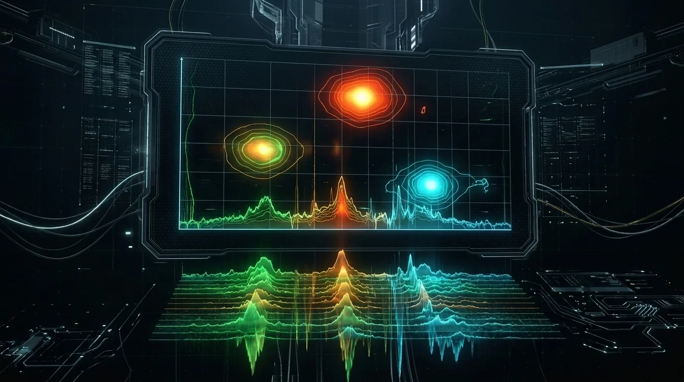 Figure: Two-dimensional target range and radial velocity heat signature produced by fast-time and slow-time 2D-FFT processing.
1
2
3
4
5
6
7
8
9
Doppler (Velocity) [m/s]
     ^
 +30 |             . (Approaching Vehicle)
     |
   0 |-------------------+------- (Static Roadside Clutter)
     |                   . (Receding Pedestrian)
 -30 |
     +-----------------------------------> Range [m]
     0        20        40        60
CFAR: Detecting Targets in Clutter
Not every peak in the Range-Doppler matrix represents a valid vehicle. Multipath reflections, asphalt scatter, and thermal noise generate false positives.
A static detection threshold would either blind the radar in clutter or trigger false alarms in open space. Radar processors implement CFAR (Constant False Alarm Rate) algorithms:
- CA-CFAR (Cell Averaging): Computes the mean noise floor across reference cells surrounding the Cell Under Test (CUT), with Guard Cells isolating target energy. A dynamic threshold is derived: $T = \alpha \cdot P_{noise}$.
- OS-CFAR (Ordered Statistic): In dense multi-target environments where adjacent targets contaminate reference cells, cells are sorted by magnitude and the $k$-th sample is selected as the baseline, preventing target masking.
6. Millimeter-Wave (77 GHz) RF & Hardware Design Challenges
The mathematical elegance of FMCW encounters unforgiving electromagnetic physics on the printed circuit board. At $77\text{ GHz}$, the free-space wavelength is just $3.9\text{ millimeters}$. Trace corners, via barrels, and solder joints act as resonant antennas and parasitics.
1. Why Standard FR-4 Fails
Standard FR-4 laminates are unusable at $77\text{ GHz}$:
- Dissipation Factor ($\tan\delta$): FR-4 exhibits a high loss tangent ($\approx 0.02$). At $77\text{ GHz}$, RF energy is dissipated as dielectric heat within millimeters.
- Dielectric Constant ($\varepsilon_r$) Inhomogeneity: Woven glass fibers embedded in epoxy resin create local variations in $\varepsilon_r$, introducing severe phase jitter and trace impedance mismatches across microstrip lines.
High-frequency automotive radar designs mandate ceramic-filled PTFE substrates such as Rogers RO3003, RO4835, or Isola Astra MT77 ($\tan\delta \approx 0.0013$). To optimize cost, manufacturers adopt Hybrid Stack-up PCBs: an ultra-thin Rogers layer on top for RF routing, bonded to standard FR-4 inner layers for digital and power distribution.
2. Skin Effect and Copper Roughness
As frequency climbs, current concentrates into an increasingly shallow depth along the conductor surface (Skin Effect). At $77\text{ GHz}$, the skin depth ($\delta$) in copper shrinks to:
\[\delta = \sqrt{\frac{\rho}{\pi f \mu}} \approx 0.23\text{ \mu m} \quad (230\text{ nm})\]When the conductor’s current-carrying cross-section is thinner than a quarter of a micron, microscopic copper foil roughness ($R_q$) forces current along a tortuous path, severely amplifying insertion loss. Radar PCBs require reverse-treated or electro-polished ultra-low profile (VLP / HVLP) copper foils.
3. TX-to-RX Isolation and Leakage
While the transmitter pumps out $+12\text{ dBm}$ of RF power, the adjacent receiver seeks to detect echoes at $-100\text{ dBm}$. Surface waves propagating across the dielectric can desensitize or saturate the LNA. Designers isolate antenna arrays with Substrate Integrated Waveguide (SIW) walls and dense ground via fences.
4. Angle of Arrival (AoA) and MIMO Architectures
A radar must resolve azimuth angle ($\theta$) alongside range and velocity. A single RX antenna lacks spatial diversity. Placing two RX antennas spaced by $d = \lambda/2$ creates a spatial phase delta ($\Delta \phi_{spatial}$):
\[\Delta \phi_{spatial} = \frac{2\pi d \sin\theta}{\lambda} = \pi \sin\theta \implies \theta = \arcsin\left( \frac{\Delta \phi_{spatial}}{\pi} \right)\]Modern automotive systems implement MIMO (Multiple-Input Multiple-Output) arrays. By time- or phase-multiplexing $N_{TX}$ transmitters across $N_{RX}$ receivers, the DSP synthesizes a Virtual Antenna Array of size $N_{TX} \times N_{RX}$. A compact transceiver with 3 TX and 4 RX antennas emulates a 12-channel physical phased-array aperture, providing sharp angular resolution without mechanical gimbals.
7. Conclusion: Transforming Waves into Geometry
The FMCW radar architecture stands as a triumph of engineering over physical measurement constraints.
Rather than chasing light pulses with nanosecond clocks, we modulate frequency to encode time. Through analog downconversion, we reduce gigahertz dynamics to audio-frequency tones, disentangle range and velocity via 2D Fourier transforms, and capture millimeter-wave signals using high-frequency PCB substrate engineering.
When torrential rain, thick fog, or pitch darkness blinds optical cameras and scatters LiDAR beams, an autonomous vehicle continues to map its environment with uncompromising fidelity. Behind that life-saving perception lies the invisible geometry of the FMCW radar.
Author: Kerem Uysal — Founder, Tech&Lab
Contact: info@keremuysal.com | info@techandlab.com